
Hey everyone!
Last articles of my mini Big Data project, and this time, after collecting the tweets and stocking them, I’ll show you an introduction of Natural Language Processing. So let’s go!
Exporting the tweets
So, do you remember when I explained to you that I’m renting a 5 (beers)€/month machine and it was cool, right? Well, it happened that because the machine has only 1 GB of rams, I’m not able to load up the JSON file into it using Python without an unpleasant

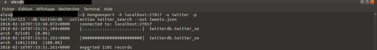
So… I’ve had to export the data first. For that, nothing too difficult (even though I spent some times searching for a solution), and since our data are into a MongoDB server, we just have to use Mongoexport! Mongoexport allows us to export our data into various type files, and among them, CSV and JSON. I could have used this format, but since you have to specify the fields to export and I didn’t know what to look for at first, I figured that it would be easier to export everything into a JSON file that I named “tweets.json” (so original, no?)
So, here it comes the time for a bit of analysis.
Time series analysis
For this part, I use the code of this book.
import sys
import json
from datetime import datetime
import matplotlib.pyplot as plt
import matplotlib.dates as mdates
import pandas as pd
import numpy as np
import pickle

with open('tweets.json', 'r') as tweets:
 all_dates = []
 for line in tweets:
 tweet = json.loads(line)
 all_dates.append(tweet.get('created_at'))
 idx = pd.DatetimeIndex(all_dates)
 ones = np.ones(len(all_dates))
First things first, the import! Since we are making a plot to show the tweet frequencies, we need to import some functions of matplotlib. We also use pandas, numpy and pickle to change the structure of the data and be able to use them for analysis.
with open('tweets.json', 'r') as tweets:
 all_dates = []
 for line in tweets:
 tweet = json.loads(line)
 all_dates.append(tweet.get('created_at'))
 idx = pd.DatetimeIndex(all_dates)
 ones = np.ones(len(all_dates))
After that, we have to open the JSON file and create a list, “all_dates” to record all the dates of present in “created_at” from the tweets. We use functions of pandas and numpy to make it readable for the future.
# the series of 1s tweets
my_series = pd.Series(ones, index=idx)
#Resampling and aggregating into 1-minute buckets
per_minute = my_series.resample('1Min').sum().fillna(0)
Here is the creation of the series that will use for the plot. Since the tweets collection was in real-time streaming, we have to aggregate them by minute for drawing the plot and make it easier to understand.
ax = plt.subplots()
ax.grid(True)
ax.set_title("Tweet Frequencies")
hours = mdates.MinuteLocator(interval=3)
date_formatter = mdates.DateFormatter('%H:%M')
datemin = datetime(2018, 2, 15, 13, 36)
datemax = datetime(2018, 2, 15, 13, 54)
ax.xaxis.set_major_locator(hours)
ax.xaxis.set_major_formatter(date_formatter)
ax.set_xlim(datemin, datemax)
max_freq = per_minute.max()
ax.set_ylim(0, max_freq)
ax.plot(per_minute.index, per_minute)
plt.savefig('tweet_time_series.png')
Final part of the code, the plot! It is possible to customize it depending on your preferences and what you want to see. Here I barely touched it, except for the datetime that I needed to change to be sure to have the right axis and a readable plot.
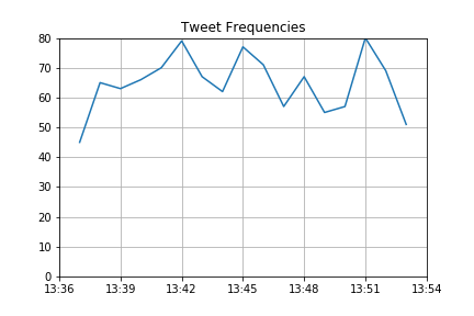
As you can see, as it is, it doesn’t show us much information because the script was launched only once, but it could be very interesting with a larger tweets dataset to see the evolution of the tweets during a particular timespan.
Text analysis
So now, after having seen the tweets frequencies, let’s see the most used hashtags.
For that, I used code found here and in the book again (both are from the same author.)
import json
from nltk.tokenize import word_tokenize
import operator
from collections import Counter
from nltk.corpus import stopwords
import string
Again, first step is the import of the modules. For the text analysis, we need to use a module use NLTK. It allows us to work with human language data in a more efficient way. Since it was the first time I used it, I had to write before the following code.
import nltk
nltk.download()
This code permits us to download and install the packages of NLTK.
import re

emoticons_str = r"""
 (?:
 [:=;] # Eyes
 [oO\-]? # Nose (optional)
 [D\)\]\(\]/\\OpP] # Mouth
 )"""

regex_str = [
 emoticons_str,
 r']+>', # HTML tags
 r'(?:@[\w_]+)', # @-mentions
 r"(?:\#+[\w_]+[\w\'_\-]*[\w_]+)", # hash-tags
 r'http[s]?://(?:[a-z]|[0-9]|[$-_@.&+]|[!*\(\),]|(?:%[0-9a-f][0-9a-f]))+', # URLs

 r'(?:(?:\d+,?)+(?:\.?\d+)?)', # numbers
 r"(?:[a-z][a-z'\-_]+[a-z])", # words with - and '
 r'(?:[\w_]+)', # other words
 r'(?:\S)' # anything else
]

tokens_re = re.compile(r'('+'|'.join(regex_str)+')', re.VERBOSE | re.IGNORECASE)
emoticon_re = re.compile(r'^'+emoticons_str+'$', re.VERBOSE | re.IGNORECASE)

def tokenize(s):
 return tokens_re.findall(s)

def preprocess(s, lowercase=False):
 tokens = tokenize(s)
 if lowercase:
 tokens = [token if emoticon_re.search(token) else token.lower() for token in tokens]
 return tokens
Here, we have to taken an consideration that a tweet is not only words but also symbols and emojis (yeah, you know, those little faces you send sometimes)!
To take them in consideration, we have to import first re and then to create the emojis. After that, we use re to tokenize the tweets which means breaking them into a list of words. If you want to know a bit more, I invite you to read this tutorial.
fname = 'tweets.json'
with open(fname, 'r') as f:
 count_all = Counter()
 for line in f:
 tweet = json.loads(line)
 # Create a list with all the terms
 terms_hash = [term for term in preprocess(tweet['text'])
 if term.startswith('#')]
 count_all.update(terms_hash)
 # Print the first 5 most frequent words
print(count_all.most_common(5))
And the final step, we have now to find all the words that begin with #. For this, we open the JSON and we use the functions we wrote just before to tokenize the words. With the help of the collection module, we can count the number of times a word appears.
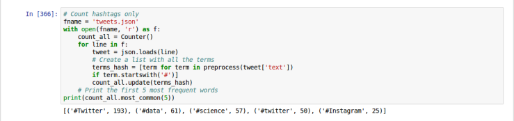
Do you remember that my keywords were “#data”, “#science”, “#twitter”, but still the first one is #Twitter with a T capital. I suppose that is a particularity of twitter that doesn’t make the difference between the lower or upper case as we can see here with #Twitter and #twitter.
Conclusion of This Mini Project
So, it’s time for the conclusion of this mini project. What did I learn doing it?
- I learnt how to configure an Ubuntu server, and use MongoDB for collecting tweets.
- I learnt how export a JSON file from MongoDB and do a little analysis of it.
- And most important, I learnt that most of the tools are available on the web but they are not all ready to use for what I want to do, and sometimes require modification to make them work according to my needs.
More than a technical aspect, I think this project was a good exercise to understand a bit more about the Big Data world, how it works and its possibilities regarding real business solving problems.
Further reflexions
Now that this mini project is over, let’s have a reflexion of what can be done after.
Indeed, I believe that many things can be done and among them:
- What about the utilization of a BI software? I believe that it is possible to use software like Tableau to read the JSON or connect a MongoDB database. Maybe it will make easier to do that kind of analysis (especially for
noobsbeginners like me)? - I think for a company it may be interesting to do that kind of analysis, especially the sentiment analysis to understand the relation between the company and its customers.
- I used twitter but I think most of the social networks can be used to do the same analysis. What if we collect all the data from various social networks and stock them into MongoDB for posterior analysis?
I’ll try to go a little bit further after with a more complete project, but the next article, ladies and gentlemen, will be a story.
Thank you for reading!
¡ Hasta luego!